Mapping Corruption in Mexico

Visualizing the Subnational Corruption Index

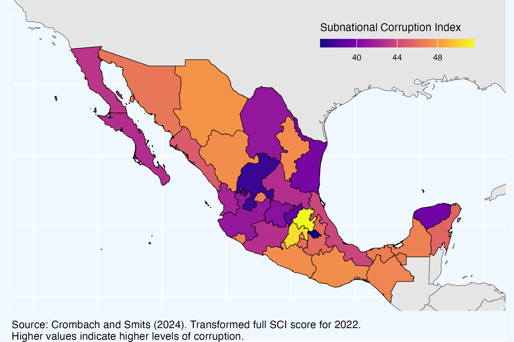
Mapping Corruption by State in Mexico in 2022

How is corruption measured here?

Corruption has many connotations and meanings. The most widely accepted definition comes from Transparency International as “the abuse of entrusted power for private gain”.

Though there are some exceptions, corruption is mostly measured through surveys on direct experiences or perceptions of corruption (Fazekas and Hernández Sánchez 2021).

In the figure above, corruption is measured from 0-100, with higher values indicating higher levels of perceived grand and petty corruption by sub-national unit in a given year.

Where does the data come from?

This map was constructed using data collected by Crombach and Smits (2024). The Subnational Corruption Database (SDC) “is constructed by combining data of 807 surveys held in the period 1995–2022 and includes the corruption experiences and perceptions of 1,326,656 respondents along 19 separate dimensions.”

The research paper which details the exact methodology can be found here and the data can be downloaded here

How was this map made?

Step 1. Load Libraries and Datasets

# Load necessary libraries
library(dplyr)          # For data manipulation
library(ggplot2)        # For creating plots
library(sf)             # For handling spatial data
library(rnaturalearth) # For fetching geographical data
library(readr)          # For reading CSV files

# Read the corruption data from a CSV file
corruption_data_full <- read_csv("data/GDL-CorruptionData-1.0.csv")

Step 2. Clean and Wrangle Data

# Filter and clean the data
corruption_subnat_mexico <- corruption_data_full %>%
  # Keep only rows for Mexico and subnational level data
  filter(iso_code == "MEX", level == "Subnat") %>%
  # Select relevant columns
  select(year, region_sci, fullsci, GDLCODE) %>%
  # Create a clean name for merging and calculate corruption index
  mutate(clean_name = stringi::stri_trans_general(region_sci, "Latin-ASCII"),
         clean_name = case_when(
           clean_name == "Michoacan de Ocampo" ~ "Michoacan",  # Correct specific region name
           TRUE ~ clean_name
         ),
         clean_name = tolower(clean_name),  # Convert names to lowercase
         corruption = 100 - fullsci)  # Calculate corruption index

# Filter the data to include only the year 2022
corruption_subnat_mexico_22 <- corruption_subnat_mexico %>%
  filter(year == 2022)

# Retrieve world map data
world <- ne_countries(scale = "medium", returnclass = "sf")

# Retrieve state-level geographical data for Mexico
subnational_mex <- ne_states(country = "Mexico", returnclass = "sf") %>%
  # Clean region names for merging
  mutate(clean_name = stringi::stri_trans_general(woe_name, "Latin-ASCII"),
         clean_name = tolower(clean_name))

Step 3. Inspect and Merge Datasets

# Inspect overlap of key variables
unique(subnational_mex$clean_name)[!unique(subnational_mex$clean_name) %in% unique(corruption_subnat_mexico$clean_name)]

# Merge geographical data with corruption data for 2022
subnational_mex <- left_join(subnational_mex, corruption_subnat_mexico_22)

Step 4. Plot!

# Create the plot
world %>%
  ggplot() +
  geom_sf() +  # Plot the world map
  geom_sf(data = subnational_mex,  # Add subnational data
          aes(fill = corruption),  # Fill regions based on corruption index
          color = "black") +  # Border color
  scale_fill_viridis_c(option = "plasma") +  # Use a color scale
  coord_sf(ylim = c(35, 15),  # Set latitude limits
           xlim = c(-120, -85)) +  # Set longitude limits
  labs(fill = "Subnational Corruption Index",  # Label for the color scale
       caption = "Source: Crombach and Smits (2024). Transformed full SCI score for 2022. \nHigher values indicate higher levels of corruption.") +  # Caption
  theme(
    panel.background = element_rect(fill = "aliceblue"),  # Background color of the plot panel
    plot.background = element_rect(fill = "aliceblue"),  # Background color of the entire plot
    legend.background = element_rect(fill = NA),  # No background for the legend
    legend.position = c(0.95, 0.95),  # Position the legend
    plot.caption = element_text(hjust = 0),  # Align caption to the left
    legend.direction = "horizontal",  # Arrange legend items horizontally
    legend.title.position = "top",  # Position legend title on top
    legend.text = element_text(size = 7),  # Text size in legend
    legend.title = element_text(size = 9),  # Title size in legend
    legend.key.height = unit(.25, "cm"),  # Height of legend keys
    legend.key.width = unit(.9, "cm"),  # Width of legend keys
    legend.justification = c(1, 1),  # Justify legend to bottom right
    panel.border = element_blank(),  # Remove panel border
    axis.ticks = element_blank(),  # Remove axis ticks
    axis.text = element_blank(),  # Remove axis text
    axis.title = element_blank(),  # Remove axis titles
    plot.margin = margin(0, 0, 0, 0)  # Remove plot margins
  )

# Export the plot to the working directory
ggsave("figures/fig-map-mex.png", width = 15, height = 10, units = "cm")

References

Crombach, Lamar, and Jeroen Smits. 2024. “The Subnational Corruption Database: Grand and Petty Corruption in 1,473 Regions of 178 Countries, 19952022.” Scientific Data 11 (1). https://doi.org/10.1038/s41597-024-03505-8.

Fazekas, Mihaly, and Alfredo Hernández Sánchez. 2021. “Emergency Procurement: The Role of Big Open Data.” In. Hart Publishing. https://doi.org/10.5040/9781509943067.ch-023.